NFL Player Analysis

Author
Affiliation

Thomas Hudson

Published

Last modified on December 10, 2024 21:04:48 Eastern Standard Time

Introduction

This is an exploration to the statistics from the 2023 NFL season. This data analysis hopes to explore different facets of the statistics provided to find common trends.

Loading Neccesary Packages

# For data manipulation and tidying
library(dplyr)

Attaching package: 'dplyr'
The following objects are masked from 'package:stats':

    filter, lag
The following objects are masked from 'package:base':

    intersect, setdiff, setequal, union
library(lubridate)

Attaching package: 'lubridate'
The following objects are masked from 'package:base':

    date, intersect, setdiff, union
library(tidyr)

#to unpack .parq files
library(arrow)

Attaching package: 'arrow'
The following object is masked from 'package:lubridate':

    duration
The following object is masked from 'package:utils':

    timestamp
# For data visualizations
library(ggplot2)

Importing the Data

All of the data can be downloaded from Kaggle. This project contains 3 data sets, the .parq files utilize the arrow package to pull the massive files into .csv files, and each file is imported and inspected independently using the read.csv() function.

#creating a .csv file for the players dataset
#this was run one time to pull the data into my folder, then reorganized
#players <- read_parquet("./competition_data/players.parq")
#write.csv(players, "players.csv", row.names = FALSE)
players <- read.csv(file = "./data/players.csv",
                    header = TRUE,
                    stringsAsFactors = FALSE)
#games <- read_parquet("./competition_data/games.parq")
#write.csv(games, "games.csv", row.names = FALSE)
games <- read.csv(file = "./data/games.csv",
                    header = TRUE,
                    stringsAsFactors = FALSE)

#plays <- read_parquet("./competition_data/plays.parq")
#write.csv(plays, "plays.csv", row.names = FALSE)
plays <- read.csv(file = "./data/plays.csv",
                    header = TRUE,
                    stringsAsFactors = FALSE)

The .parq files will not be included in the github for this project due to the size of the files being too large.

Data Structures and Variables

players

Rows: 1,683
Columns: 7
$ nflId       <int> 25511, 29550, 29851, 30842, 33084, 33099, 33107, 33130, 33…
$ height      <dbl> 6.333, 6.333, 6.167, 6.500, 6.333, 6.500, 6.333, 5.833, 6.…
$ weight      <int> 225, 328, 225, 267, 217, 245, 315, 175, 300, 222, 220, 229…
$ birthDate   <chr> "1977-08-02 20:00:00", "1982-01-21 19:00:00", "1983-12-01 …
$ collegeName <chr> "Michigan", "Arkansas", "California", "UCLA", "Boston Coll…
$ position    <chr> "QB", "T", "QB", "TE", "QB", "QB", "T", "WR", "DE", "QB", …
$ displayName <chr> "Tom Brady", "Jason Peters", "Aaron Rodgers", "Marcedes Le…

There are 7 variables in the data players data frame:

  1. nflId: Unique identifier for the player.

  2. height: Height of the player in feet.

  3. weight: Weight of the player in pounds.

  4. birthDate: Player’s date of birth (some missing values).

  5. collegeName: The college the player attended.

  6. position: The player’s position in the team (e.g., QB, T, TE).

  7. displayName: The player’s name.

games

glimpse(games)
Rows: 136
Columns: 8
$ gameId            <int> 2022090800, 2022091100, 2022091101, 2022091102, 2022…
$ season            <int> 2022, 2022, 2022, 2022, 2022, 2022, 2022, 2022, 2022…
$ week              <int> 1, 1, 1, 1, 1, 1, 1, 1, 1, 1, 1, 1, 1, 1, 1, 1, 2, 2…
$ homeTeamAbbr      <chr> "LA", "ATL", "CAR", "CHI", "CIN", "DET", "HOU", "MIA…
$ visitorTeamAbbr   <chr> "BUF", "NO", "CLE", "SF", "PIT", "PHI", "IND", "NE",…
$ homeFinalScore    <int> 10, 26, 24, 19, 20, 35, 20, 20, 9, 28, 21, 24, 23, 2…
$ visitorFinalScore <int> 31, 27, 26, 10, 23, 38, 20, 7, 24, 22, 44, 19, 7, 21…
$ gameDatetime      <chr> "2022-09-08 16:20:00", "2022-09-11 09:00:00", "2022-…

There are 8 variables in the games data set

  1. gameId: A unique identifier for each game.

  2. season: The year of the season during which the game was played.

  3. week: The week number of the NFL season.

  4. homeTeamAbbr: The abbreviation of the home team’s name.

  5. visitorTeamAbbr: The abbreviation of the visiting team’s name.

  6. homeFinalScore: The final score of the home team.

  7. visitorFinalScore: The final score of the visiting team.

  8. gameDatetime: The date and time when the game occurred.

plays

glimpse(plays)
Rows: 12,486
Columns: 35
$ gameId                           <int> 2022100908, 2022091103, 2022091111, 2…
$ playId                           <int> 3537, 3126, 1148, 2007, 1372, 2165, 2…
$ ballCarrierId                    <int> 48723, 52457, 42547, 46461, 47857, 54…
$ ballCarrierDisplayName           <chr> "Parker Hesse", "Chase Claypool", "Da…
$ playDescription                  <chr> "(7:52) (Shotgun) M.Mariota pass shor…
$ quarter                          <int> 4, 4, 2, 3, 2, 3, 4, 1, 2, 3, 3, 3, 4…
$ down                             <int> 1, 1, 2, 2, 1, 3, 3, 1, 1, 1, 3, 3, 3…
$ yardsToGo                        <int> 10, 10, 5, 10, 10, 17, 5, 10, 10, 10,…
$ possessionTeam                   <chr> "ATL", "PIT", "LV", "DEN", "BUF", "AT…
$ defensiveTeam                    <chr> "TB", "CIN", "LAC", "LV", "TEN", "CAR…
$ yardlineSide                     <chr> "ATL", "PIT", "LV", "DEN", "TEN", "AT…
$ yardlineNumber                   <int> 41, 34, 30, 37, 35, 18, 25, 25, 40, 2…
$ gameClock                        <chr> "00:07:52", "00:07:38", "00:08:57", "…
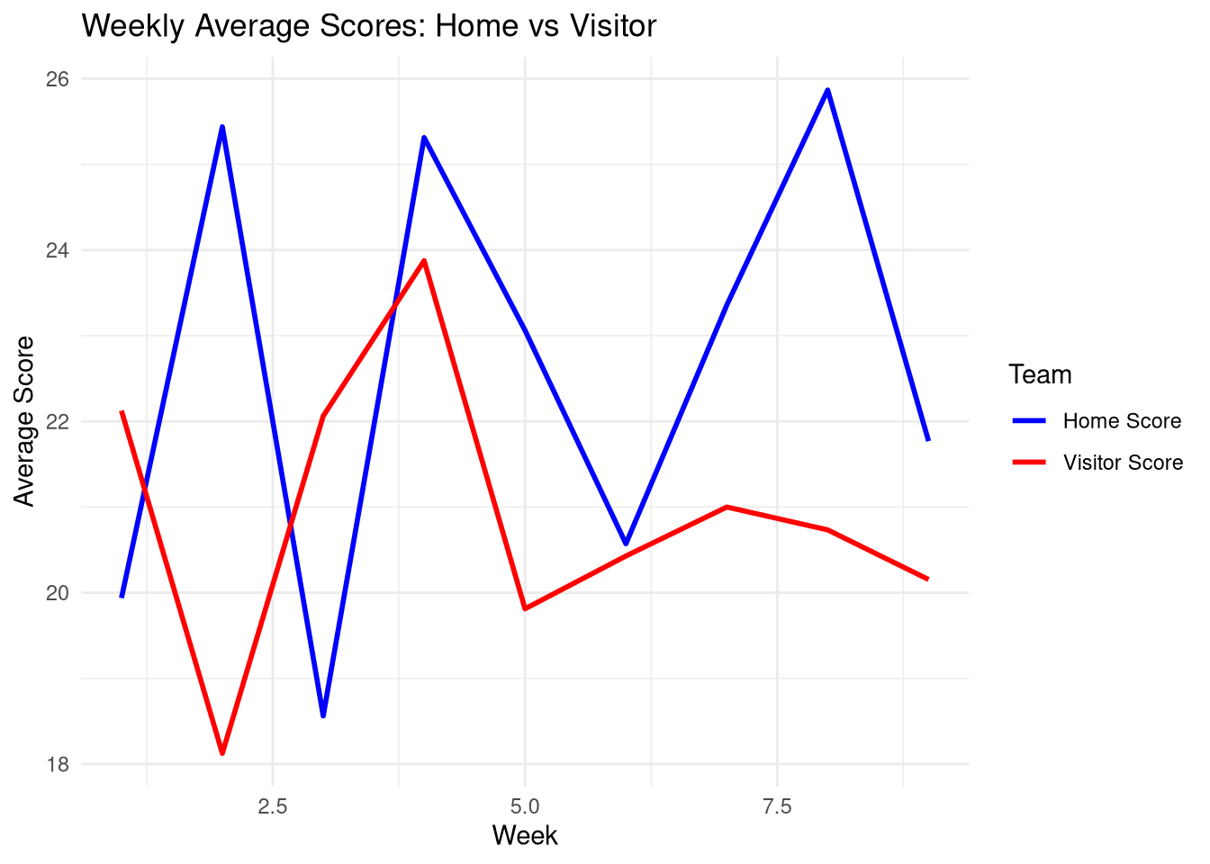
$ preSnapHomeScore                 <int> 21, 14, 10, 19, 7, 14, 17, 0, 13, 23,…
$ preSnapVisitorScore              <int> 7, 20, 3, 16, 7, 13, 24, 0, 7, 27, 0,…
$ passResult                       <chr> "C", NA, "C", NA, NA, "C", "R", NA, N…
$ passLength                       <int> 6, NA, 11, NA, NA, -5, NA, NA, NA, -5…
$ penaltyYards                     <int> NA, NA, NA, NA, NA, NA, NA, NA, NA, N…
$ prePenaltyPlayResult             <int> 9, 3, 15, 7, 3, 5, 3, 7, 9, 3, 3, 5, …
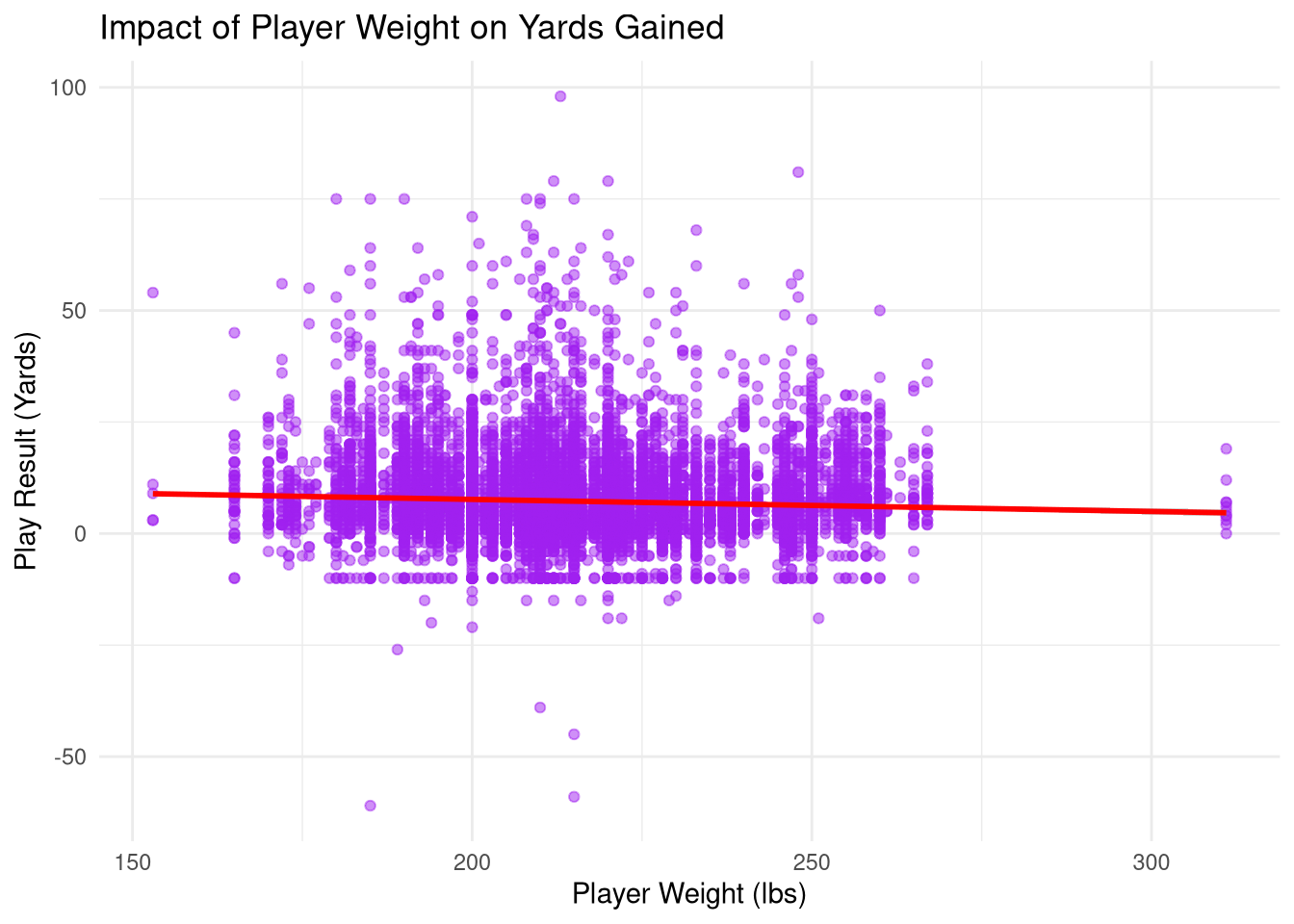
$ playResult                       <int> 9, 3, 15, 7, 3, 5, 3, 7, 9, 3, 3, 5, …
$ playNullifiedByPenalty           <chr> "N", "N", "N", "N", "N", "N", "N", "N…
$ absoluteYardlineNumber           <int> 69, 76, 40, 47, 75, 28, 85, 85, 70, 8…
$ offenseFormation                 <chr> "SHOTGUN", "SHOTGUN", "I_FORM", "SING…
$ defendersInTheBox                <int> 7, 7, 6, 6, 7, 5, 4, 7, 6, 7, 6, 6, 6…
$ passProbability                  <dbl> 0.7472844, 0.4164537, 0.2679328, 0.59…
$ preSnapHomeTeamWinProbability    <dbl> 0.976784671, 0.160484683, 0.756661031…
$ preSnapVisitorTeamWinProbability <dbl> 0.02321533, 0.83951532, 0.24333897, 0…
$ homeTeamWinProbabilityAdded      <dbl> -0.006110488, -0.010864805, -0.037408…
$ visitorTeamWinProbilityAdded     <dbl> 0.006110488, 0.010864805, 0.037408687…
$ expectedPoints                   <dbl> 2.3606089, 1.7333441, 1.3128546, 1.64…
$ expectedPointsAdded              <dbl> 0.98195511, -0.26342389, 1.13366620, …
$ foulName1                        <chr> NA, NA, NA, NA, NA, NA, NA, NA, NA, N…
$ foulName2                        <chr> NA, NA, NA, NA, NA, NA, NA, NA, NA, N…
$ foulNFLId1                       <int> NA, NA, NA, NA, NA, NA, NA, NA, NA, N…
$ foulNFLId2                       <int> NA, NA, NA, NA, NA, NA, NA, NA, NA, N…

There are 35 variables in the games data set

  1. gameId: Unique identifier for the game.

  2. playId: Unique identifier for the play within the game.

  3. ballCarrierId: NFL ID of the ball carrier during the play (if applicable).

  4. ballCarrierDisplayName: Name of the ball carrier during the play (if applicable).

  5. playDescription: Textual description of the play, including actions and results.

  6. quarter: The quarter of the game when the play occurred.

  7. down: The down number during the play (e.g., 1st, 2nd).

  8. yardsToGo: The number of yards needed for a first down at the start of the play.

  9. possessionTeam: The team that possessed the ball during the play.

  10. defensiveTeam: The team defending during the play.

  11. yardlineSide: The side of the field where the play started, based on the team.

  12. yardlineNumber: The specific yard line where the play started.

  13. gameClock: The time remaining in the game during the play (in MM:SS).

  14. preSnapHomeScore: The home team’s score before the play began.

  15. preSnapVisitorScore: The visiting team’s score before the play began.

  16. passResult: Outcome of the pass play (if applicable, e.g., completed, intercepted).

  17. passLength: Distance of the pass in yards (if applicable).

  18. penaltyYards: The number of yards gained or lost due to penalties (if applicable).

  19. prePenaltyPlayResult: Outcome of the play before accounting for penalties (in yards).

  20. playResult: Final outcome of the play, including penalty effects (in yards).

  21. playNullifiedByPenalty: Indicator of whether the play was nullified due to a penalty.

  22. absoluteYardlineNumber: Standardized yard line on the field where the play began.

  23. offenseFormation: The offensive team’s formation during the play (e.g., shotgun).

  24. defendersInTheBox: The number of defensive players positioned near the line of scrimmage.

  25. passProbability: Probability of a pass play based on pre-play context.

  26. preSnapHomeTeamWinProbability: The home team’s likelihood of winning before the play.

  27. preSnapVisitorTeamWinProbability: The visiting team’s likelihood of winning before the play.

  28. homeTeamWinProbabilityAdded: Change in the home team’s win probability due to the play.

  29. visitorTeamWinProbabilityAdded: Change in the visiting team’s win probability due to the play.

  30. expectedPoints: The expected points based on field position before the play.

  31. expectedPointsAdded: Change in expected points due to the play.

  32. foulName1: Name of the first foul committed during the play (if applicable).

  33. foulName2: Name of the second foul committed during the play (if applicable).

  34. foulNFLId1: NFL ID of the player who committed the first foul (if applicable).

  35. foulNFLId2: NFL ID of the player who committed the second foul (if applicable).

Data Visualization

Exploring the games Dataset

Home Team Advantage?

First thing I as hoping to analyze was whether the home team truely had an advantage.

Figure 1: line graph that compares the average scores of home and visiting teams across weeks or seasons.

Generally, the home team scored more points than the visiting team.

Close games vs. Blow outs

I also want to figure out what is a “normal margin of vistory in a game. Do teams normally win by a lot of points, or is there some score that is more common than others.

Figure 2: Histogram that analyzes the distribution of score differences

By far, the most common margin of victory/defeat is 3 points, which is equivaalent to 1 field goal. It also appears that after about 10 points, the margins occur just about as often as each other, all 5 or less times, with a few outlier differences past 24.

Exploring the plays data set

Play Outcome by Formation

I want to figure out which formations lead to the most positive results

Figure 3: Bar graph analyzing yards per play by formation

It seems that the formations that utilize 0 or 1 runningbacks (empty, shotgun, singleback) end up averaging more yards than formations with 2 or more running backs. This can be very circumsatntial, as those plays may be run in “passing obvious” situations where the defending team is simply trying to prevent a big play, where as heavier formations will be used in short yardage situations to guarentee positive gains without the inherent risk of an incomplete or intercepted pass.

Defenders in the box vs. position on the field

“The box” on defense refers to the area on the field between the edge of the down linemen, withing about 5-7 yards of the line of scrimmage. This often is to ensure a strong run defense at the cost of bigger, less mobile players having to be in pass coverage. This chart looks to figure out if there is a corelation between position on the field and how many defenders are in the box.

Warning: Removed 5 rows containing non-finite outside the scale range
(`stat_binhex()`).
`geom_smooth()` using formula = 'y ~ x'
Warning: Removed 5 rows containing non-finite outside the scale range
(`stat_smooth()`).

Figure 4: hexagonal point graph for yardline number against defenders in the box.

This graph shows us that generally, teams mostly use between 5 players in the box (most often referred to as “dime package”) and 8 players in the box (which is just 8-in-the box). There seems to be a slightly negative trend in yard line number and defenders in the box, meaning that there is some correlation between the start of the play on th field, and defenders in the box.

Combined Analysis

Player Attributes and Play Success

This graph aims to analyze what is th “ideal” player weight in terms of yards gained per carry.

`geom_smooth()` using formula = 'y ~ x'

Figure 5: scatter plot with the weight of every player who has carried the ball, and how many yars were gained on that attempt

This shows that on average, there is not a lot of correlation between weight, and being a better ball carrier, but it appear that players between 180 and 230 lbs account for the most big gains, with it being somewhat more frequent as you get closer to the middle at about 210.

College Representation and Game Impact

This graph looks to analyze which colleges produce the players with the most positive game impact

scoring_plays <- combined_data %>%
  filter(playResult > 0) %>%
  group_by(collegeName) %>%
  summarize(total_yards = sum(playResult, na.rm = TRUE)) %>%
  arrange(desc(total_yards)) %>%
  top_n(10, total_yards)

# Bar chart for colleges
ggplot(scoring_plays, aes(x = reorder(collegeName, total_yards), y = total_yards)) +
  geom_bar(stat = "identity", fill = "orange") +
  coord_flip() +
  labs(title = "Top Colleges Contributing to Scoring Plays",
       x = "College", y = "Total Yards Gained") +
  theme_minimal()

Alabama has produced the most yards by a substantial margin compared to the rest of country. The South Eastern Conference (SEC) also accounts for the rest of the top 4, and 7 of the total schools shown above. These schools have been the most successful at producing players to go to the NFL, and having players then have a positive impact on those games.